Learning Collection

Exploring the Distribution of Urban Community Gardens Among New York City Boroughs through R and Spatial Data Visualization

In this tutorial, we will explore how to analyze urban community gardening distribution across different boroughs using R and spatial data analysis techniques. We will use the sf, tidyverse, and ggplot2 libraries to load, clean, and visualize the required data. Let’s begin by setting up the environment and loading the necessary libraries.

# Required Libraries
library(sf)
library(dplyr)
library(ggplot2)
library(readxl)
library(leaflet)

Load the dataset and convert multipolygons to an sf object:

We start by reading the GreenThumb_Garden_Info.csv file containing information about the locations of community gardens and converting the ‘multipolygon’ field to an sf object.

Data source: https://data.cityofnewyork.us/dataset/GreenThumb-Garden-Info/p78i-pat6/data

Load the borough shapefile and perform spatial join

Next, we load the borough boundaries shapefile, transform its Coordinate Reference System (CRS), and perform a spatial join with the garden data.

# Load the borough shapefile and transform the CRS
borough_shapefile <- st_read('C:/Users/Zobaer Ahmed/Documents/Zobaer_github_page/portfolio/shapefile/Borough Boundaries/geo_export_2097f264-292b-4741-b4bd-9b58f6a775b2.shp')

Reading layer `geo_export_2097f264-292b-4741-b4bd-9b58f6a775b2' from data source `C:\Users\Zobaer Ahmed\Documents\Zobaer_github_page\portfolio\shapefile\Borough Boundaries\geo_export_2097f264-292b-4741-b4bd-9b58f6a775b2.shp' 
  using driver `ESRI Shapefile'
Simple feature collection with 5 features and 4 fields
Geometry type: MULTIPOLYGON
Dimension:     XY
Bounding box:  xmin: -74.25559 ymin: 40.49613 xmax: -73.70001 ymax: 40.91553
Geodetic CRS:  WGS84(DD)

borough_shapefile <- st_transform(borough_shapefile, crs = st_crs(garden_data_sf))

# Perform spatial join
joined_data <- st_join(borough_shapefile, garden_data_sf, join = st_intersects)

Calculate the number of gardens per borough and merge the result back into the shapefile

Now, let us calculate the number of gardens present in each borough and merge the result back into the shapefile.

# Count the number of gardens in each borough
borough_garden_count <- joined_data %>%
  group_by(boro_name.x) %>%
  summarise(count = n()) 

# Convert the garden count to a regular data frame
borough_garden_count_df <- as.data.frame(borough_garden_count)

# Merge the count data back into the borough shapefile
borough_shapefile <- borough_shapefile %>%
  left_join(borough_garden_count_df, by = c("boro_name" = "boro_name.x"))

Plot the map with borough names and garden counts

Now, we create maps illustrating the distribution of gardens across different boroughs along with their respective counts.

# Calculate the centroids of each borough for labeling
centroids <- st_centroid(borough_shapefile)

Warning: st_centroid assumes attributes are constant over geometries

# Extract coordinates for labels
borough_labels <- data.frame(st_coordinates(centroids))

# Add borough names to the labels data frame
borough_labels$boro_name <- borough_shapefile$boro_name

# Plot the map with borough names
ggplot(data = borough_shapefile) +
  geom_sf(aes(fill = count), color = 'black') +
  geom_text(data = borough_labels, aes(X, Y, label = boro_name), check_overlap = TRUE, nudge_y = 0.02) +
  scale_fill_viridis_c() +
  labs(title = 'Distribution of Gardens Across Different Boroughs',
       fill = 'Number of Gardens') +
  theme_minimal()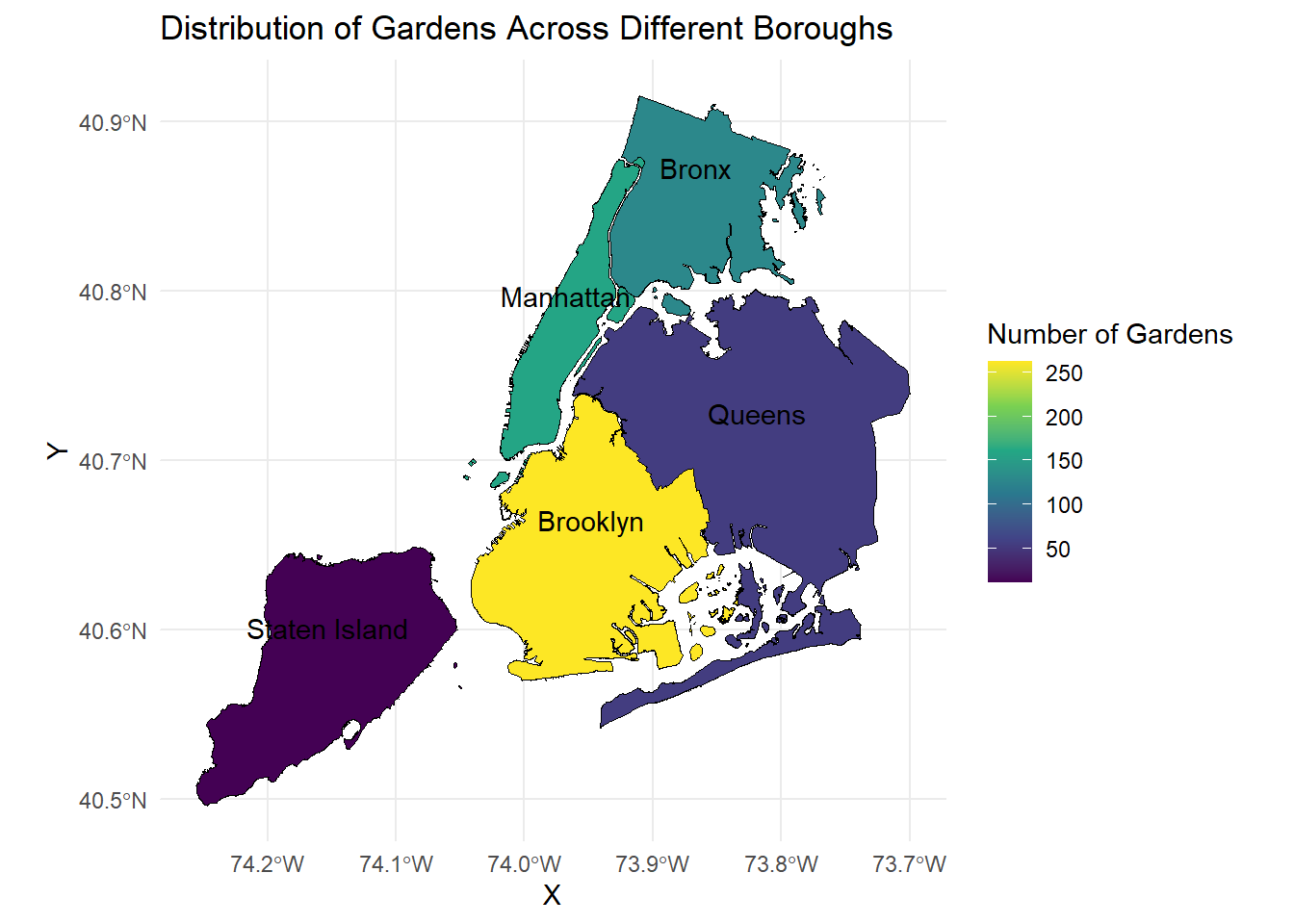

Spatial Density of Gardens

This code generates a base map showing the borough shapes filled with white colors and outlines drawn in black. The red dots represent the location of individual community gardens overlaid on top of the borough boundaries. This plot aims to display the overall spatial distribution of gardens within the study area.

ggplot() +
  geom_sf(data = borough_shapefile, fill = 'white', color = 'black') +
  geom_sf(data = garden_data_sf, color = "red", size = 0.5, alpha = 0.6) +
  labs(title = "Spatial Density of Gardens") +
  theme_minimal()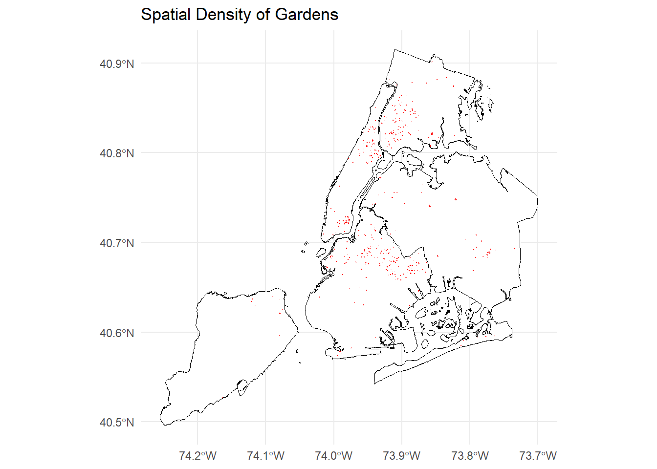

Distribution and Number of Urban Community Gardens Across Different Boroughs - Basic Version

The following code creates a thematic map where each borough shape is filled according to the number of gardens it contains. Additionally, individual garden points are shown as transparent red dots. This plot visually represents both the total number of gardens and their distribution among various boroughs.

ggplot() +
  geom_sf(data = borough_shapefile, aes(fill = count), color = 'black') + # Boroughs colored by garden count
  geom_sf(data = garden_data_sf, color = "red", size = 0.5, alpha = 0.6) + # Garden points
  geom_text(data = borough_labels, aes(X, Y, label = boro_name), check_overlap = TRUE, nudge_y = 0.02) + # Borough labels
  scale_fill_viridis_c() + # Color scale for boroughs
  labs(title = 'Distribution and Number of Urban Community Gardens Across Different Boroughs',
       fill = 'Number of Gardens') +
  theme_minimal()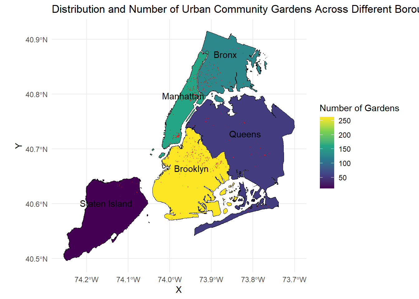

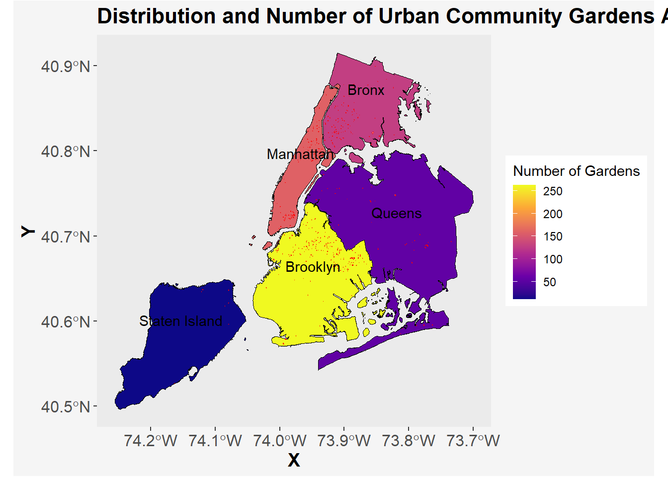
Distribution and Number of Urban Community Gardens Across Different Boroughs - Enhanced Version

Similar to the previous example, but with larger garden point sizes and customized color palette for better visual representation.

ggplot() +
  geom_sf(data = borough_shapefile, aes(fill = count), color = 'black') + # Boroughs colored by garden count
  geom_sf(data = garden_data_sf, color = "red", size = 2, alpha = 0.8) + # Garden points with increased size
  geom_text(data = borough_labels, aes(X, Y, label = boro_name), check_overlap = TRUE, nudge_y = 0.02) + # Borough labels
  scale_fill_viridis_c(option = "C") + # Custom color scale for boroughs
  labs(title = 'Distribution and Number of Urban Community Gardens Across Different Boroughs',
       fill = 'Number of Gardens') +
  theme(
    axis.text.x = element_text(size = 12),
    axis.text.y = element_text(size = 12),
    axis.title = element_text(size = 14, face = "bold"),
    plot.title = element_text(size = 16, face = "bold"),
    plot.caption = element_text(size = 10),
    plot.background = element_rect(fill = "#f5f5f5"),
    panel.grid = element_blank()
  )

Converting Multi-Part Geometries to Single-Part and Creating a Leaflet Map

This code snippet performs two main tasks: first, it converts the multi-part geometry columns of the garden_data_sf sf object into single-point geometries; secondly, it creates an interactive leaflet map displaying markers at each garden location.

Step 1: Converting Multi-Part Geometries to Single-Part

To ensure that our subsequent analyses or visualizations work correctly, especially when dealing with specific functions like clustering or distance calculations, it’s often beneficial to have single-part geometries instead of multi-part ones. Here, we convert the multi-geometry column of the garden_data_sf data frame into separate single-point geometries using the st_cast() function.

# Convert multi-part geometries to single-part
garden_data_single <- st_cast(garden_data_sf, "POINT")

Warning in st_cast.sf(garden_data_sf, "POINT"): repeating attributes for all
sub-geometries for which they may not be constant

Step 2: Creating a Regular Data Frame and Longitude-Latitude Columns

After converting the multi-part geometries to single-parts, we extract the longitude and latitude values into new columns called lon and lat. These columns will later serve as input variables for creating the leaflet map.

# Create a regular data frame from the sf object
garden_data_df <- as.data.frame(garden_data_single)

# Extract longitude and latitude
garden_data_df$lon <- st_coordinates(garden_data_single)[, 'X']
garden_data_df$lat <- st_coordinates(garden_data_single)[, 'Y']

Step 3: Creating a Leaflet Map

Finally, we utilize the leaflet package to generate an interactive map displaying markers at every garden location based on the extracted longitude and latitude columns.

# Create a leaflet map
leaflet(garden_data_df) %>%  
  addTiles() %>%             # Add default OpenStreetMap tiles
  addMarkers(                 # Add markers to the map
              lng = ~lon,      # Set longitude as marker position x coordinate
              lat = ~lat,      # Set latitude as marker position y coordinate
              popup = ~gardenname # Display garden name as marker popup text
            )

This code results in an engaging, dynamic map that allows users to interactively inspect the locations of all community gardens in the dataset.

Enjoyed the tutorial? Consider fueling my efforts with a coffee!